How to maximise profits by better production planning - Part 2

23 November 2017

Introduction

In the first part of this two part white paper we looked at:

The basic principles of Operational Planning; balancing Capacity and Demand
The challenges to achieving effective planning
How to determine the most appropriate planning horizon and units to be used

Probably the most important point to come out of the first part though was that it is necessary to identify the constraint resource and use that as the basis for defining the capacity.

In this second part we will look at how to define Capacity and Demand and then look at the types of tools which are required to support the planning process.

Capacity Definition

Once the granularity of the plan has been defined and the constraint has been determined, as discussed in the first part of this paper, it is necessary to decide how to define the capacity of each time bucket. Typically a constraint resource will only be available to process products for part of the time it is available.

For example if the constraint is a machine, it will be unavailable for processing when it is undergoing maintenance, when it is changing over from one product to another and when it is broken down. Typically the rate at which a machine, particularly a sophisticated bespoke machine, will process products will vary. Defining the capacity of a constraint resource is therefore not a straightforward process. The difference between adopting an optimistic and a pessimistic capacity can have a significant impact on a plan.

Some general guidelines are:

Exclude known periods when the resource will definitely not be available. For example a maintenance period
Use an average value of availability based on historic data. In situations where historic data is not available it will be necessary to use an estimate of the capacity as this will be better than not planning at all. At the same time making sure that data capture is started as soon as possible.
As we discussed in the first part, it is important to ensure that the basis used for defining capacity is the same as that used for demand. It’s important that both capacity and demand are expressed in the same terms e.g. for a business producing cars it is no use saying there is a demand for 500 cars per month and there is a capacity of 80 hours per week. We need to say there is a demand of 500 cars per month and there is a capacity to produce 600 cars per month.
Update the capacity figures as more actual data becomes available

Forecasting Demand

As discussed in part 1 the operational planning process needs to start well in advance of customers placing orders for products. At least part of the demand will normally, therefore, be in the form of a forecast.

There are many methods for forecasting and it is not possible in this paper to investigate them in detail. Broadly speaking there are two methods. Where demand is generally stable and predictable it is possible to use statistical methods to predict future demand based on recent history. Where the demand is not stable or predictable it is necessary to rely on predictions from customer-facing individuals in the business as to what customers are likely to require.

Whichever method is used it is important that sufficient effort is invested in the forecasting process to ensure that the results are as accurate as possible. As part of this process it is important that the forecast is reviewed on a regular basis.

It is also important to recognise that forecasting is not about predicting a single figure for a particular product in a particular period. That is almost certainly what will not happen! There are simple statistical methods which can be used to predict the probability of future demand falling within a given range. A product whose demand has varied by ± 30% in the past will have a much wider range for a given probability than one whose demand varies by ± 10%.

This approach can be very useful in a make to stock environment as it can be used as the basis for how much safety stock is required. The product with the higher variability will require significantly more safety stock to protect against probable future variations in demand.

Demand Conversion

The forecast demand will typically be expressed in the quantity of a particular product being required. As discussed above, for planning purposes, this needs to be converted into the same units as the capacity.

So as well as identifying which resource is the constraint within a facility we need to know how much time each product will require on the constraint. It is important that the data is accurate and defined on the same basis as the capacity.

As with capacity the time taken to produce a product may vary considerably between different periods.

Some general guidelines are:

Only include the time the product will spend on the resource. Do not include waiting time or travel time.
Use an average value based on historic data. As with capacity it is perfectly acceptable to use an estimated figure if historic data is not available. It is also important to start capturing data as soon as possible.
Update the process times on a regular basis as more actual data becomes available

Planning Tools - Demand Loading

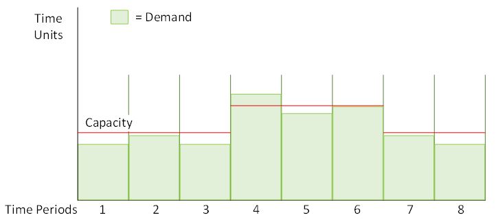
Ideally a planning tool will produce an accurate view of the loading of demand against capacity in order that periods where demand exceeds or is very close to capacity can be readily identified.

As demand will be defined in the same units as capacity this is, on the face of it, a relatively easy task.

However, there is the question of which bucket to put the demand in. In a simple case where a product is produced on a single resource we could put the demand in the period in which it is due for delivery. Where there is a relatively long lead time for the process after the constraint it may be necessary to offset the delivery period by that lead time in order to present an accurate picture of loading on the constraint. It is also possible that products may be required at the beginning of the period and there is no guarantee that it would be produced by then. Therefore it would be advisable to place it in the period before it is due.

For a long lead time environment where the time buckets are in months the situation would be similar to this:

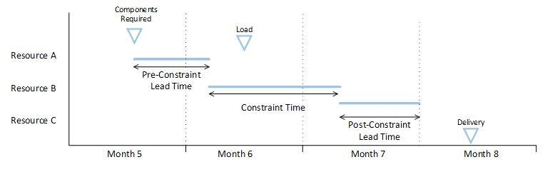
In the example above Resource B is the constraint. The time spent in the facility before and after the constraint are identified as the ‘Pre-Constraint Lead Time’ and ‘Post-Constraint Lead Time’ respectively. The time spent on the constraint is known as the ‘Constraint Time’ and effectively represents the demand.

In establishing which time bucket the demand should be loaded into we need to work backwards in time from the Delivery Date.

As the demand needs to be delivered in month 8 we start our calculation in month 7 and adding together the Post-Constraint Lead Time and the Constraint Time we can see that the demand needs to be loaded in month 6.

In the case where this demand requires one or more components which are made in other facilities we also need to establish a ‘delivery date’ for those components. The above diagram indicates that the plan would require production on resource A to start in month 5. The calculation for the location of demand for the components would then need to start in month 4.

The detailed calculation of this loading process also needs to take account of the availability of components currently held in stock. If the calculation identifies a requirement for a quantity of a particular component and there is at least that quantity of the component in stock then the calculation does not need to continue.

Planning Tools - Load Smoothing

In the earlier example of demand loading it was evident that the demand in period 4 exceeded the available. This has been highlighted in the version below.

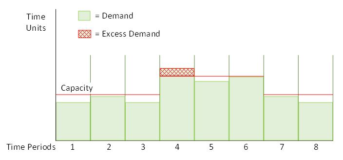
This is clearly an impractical plan because, if it were implemented, there is a strong possibility that required delivery dates would not be met. There are a number of ways in which this overload could be removed and the plan made achievable:

Increase the capacity in that period
Reduce the demand
Negotiate a later delivery date
Plan to make the demand earlier

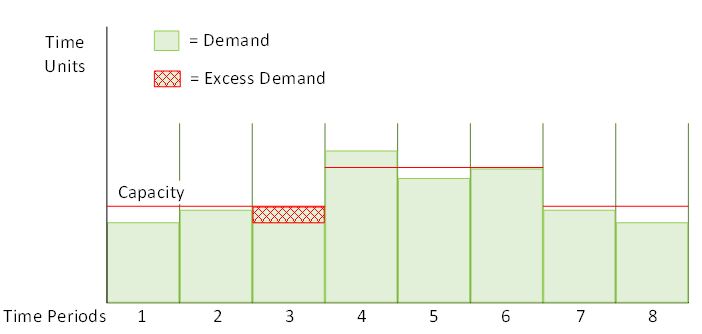
The last option can be achieved within the planning tool if it is able to implement load smoothing. This entails identifying overloaded time periods and then moving the overload to an earlier period. This can be made more sophisticated by giving different priorities to the products making up the demand. So instead of moving the element of demand that happens to exceed capacity, the product with the lowest priority is moved.

An illustration of the completed plan is given in the following diagram.

It is quite possible that the excess demand cannot be smoothed out in this way because there is simply not enough capacity ahead of when the demand is required. In this situation it is necessary to either increase the capacity or reduce the demand to ensure that customer service and quality is not compromised.

As we highlighted in part 1 it is very important that demand overloads are identified as early as possible in the planning process. The earlier they are identified the more flexibility there is to manage the capacity/demand relationship.

Conclusion

This paper has merely scratched the surface of what is a wide ranging and complex subject. In particular we have not attempted the many different types of business for which the planning process is critical, but may not be performed effectively.

If you would like to discuss your particular planning issues, or to see case studies where improved production planning has led to better profitability, please visit our website or contact Argenta, who will be happy to help.

Back to Blog listings

blog